45 change order of data labels in excel chart
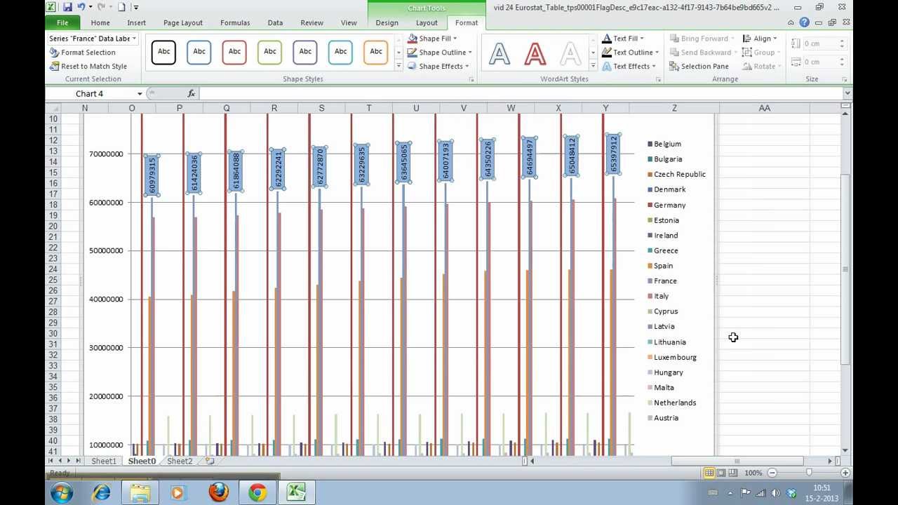
Change order of data labels in chart - Microsoft Community Yes No TA tartan10 Replied on March 4, 2013 In reply to Ty_hell_heaven's post on March 4, 2013 The data were added in the order shown in the list before realizing that the labels could not be moved around. The order of the labels on the right should be, downward, 10, 8, 6, 4, and 2. Report abuse Was this reply helpful? Yes No TA tartan10 How to Create and Customize a Treemap Chart in Microsoft Excel Simply click that text box and enter a new name. Next, you can select a style, color scheme, or different layout for the treemap. Select the chart and go to the Chart Design tab that displays. Use the variety of tools in the ribbon to customize your treemap. For fill and line styles and colors, effects like shadow and 3-D, or exact size and ...
How to change the Data Label Order in a Column Chart. - Power BI In this scenario, if you want to modify the Legend order, you would need to create separate measures to calculate the results for each type of Business Unit, then place each measure in the Values area in order you wish. For more details, please review this similar thread, it works for column chart. Thanks, Lydia Zhang
Change order of data labels in excel chart
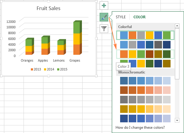
How to add or move data labels in Excel chart? - ExtendOffice In Excel 2013 or 2016. 1. Click the chart to show the Chart Elements button . 2. Then click the Chart Elements, and check Data Labels, then you can click the arrow to choose an option about the data labels in the sub menu. See screenshot: In Excel 2010 or 2007. 1. click on the chart to show the Layout tab in the Chart Tools group. See ... How to reorder chart series in Excel? - ExtendOffice Right click at the chart, and click Select Data in the context menu. See screenshot: 2. In the Select Data dialog, select one series in the Legend Entries (Series) list box, and click the Move up or Move down arrows to move the series to meet you need, then reorder them one by one. 3. Click OK to close dialog. Change the Order of Data Series of a Chart in Excel - Excel Unlocked We can change this order. Right click on this chart and click on the Select Data option. After that select 2019 from the data series and click on the down arrow. This will move the data series 2019 below 2020. Click OK. As a result, you would see a change of order in your column chart as follows. This brings us to the end of the blog.
Change order of data labels in excel chart. How to Change Excel Chart Data Labels to Custom Values? Now, click on any data label. This will select "all" data labels. Now click once again. At this point excel will select only one data label. Go to Formula bar, press = and point to the cell where the data label for that chart data point is defined. Repeat the process for all other data labels, one after another. See the screencast. Points to note: Changing the order of items in a chart - PowerPoint Tips Blog 2. Individually change the order of items. You can manage the order of items one by one if you don't want to reverse the entire set. Follow these steps: With the chart selected, click the Chart Tools Design tab. Choose Select Data in the Data section. The Select Data Source dialog box opens. You can only change the values on the left side of ... How to change the order of your chart legend - Excel Tips & Tricks ... Under the Data section, click Select Data. Step 2: In the Select Data Source pop up, under the Legend Entries section, select the item to be reallocated and, using the up or down arrow on the top right, reposition the items in the desired order. How to change the order of data layer on chart - MrExcel Message Board #1 Hi -- I have 3 series, and on the line chart, two of the series cover a very similar path. I need the series that's currently behind the other to come up front. I've tried series order on data formatting, but it only changes the Legend presentation, not how the data is displayed. Thanks, Wade [/img] Excel Facts Excel Wisdom
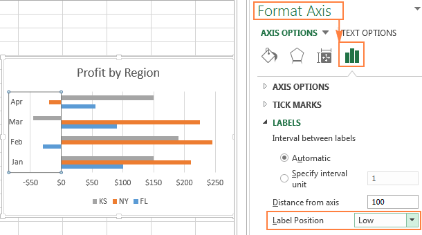
How to add data labels from different column in an Excel chart? Right click the data series in the chart, and select Add Data Labels > Add Data Labels from the context menu to add data labels. 2. Click any data label to select all data labels, and then click the specified data label to select it only in the chart. 3. Change the labels in an Excel data series | TechRepublic Click the Chart Wizard button in the Standard toolbar. Click Next. Click the Series tab. Click the Window Shade button in the Category (X) Axis Labels box. Select B3:D3 to select the labels in your... How to rotate axis labels in chart in Excel? - ExtendOffice 1. Go to the chart and right click its axis labels you will rotate, and select the Format Axis from the context menu. 2. In the Format Axis pane in the right, click the Size & Properties button, click the Text direction box, and specify one direction from the drop down list. See screen shot below: How to reverse order of items in an Excel chart legend? Right click the chart, and click Select Data in the right-clicking menu. See screenshot: 2. In the Select Data Source dialog box, please go to the Legend Entries (Series) section, select the first legend ( Jan in my case), and click the Move Down button to move it to the bottom. 3.
Change the format of data labels in a chart To get there, after adding your data labels, select the data label to format, and then click Chart Elements > Data Labels > More Options. To go to the appropriate area, click one of the four icons ( Fill & Line, Effects, Size & Properties ( Layout & Properties in Outlook or Word), or Label Options) shown here. Sort legend items in Excel charts - teylyn Finally, go back to the data for the helper series up in I2 to I5 and change the values for the helper series to zeros. Now your chart should look like this: step 6. Result: The series order is yellow, blue, pink, green, but the legend items are sorted alphabetically, i.e. apples - pink. bananas - green. Is there a way to change the order of Data Labels? Answer Rena Yu MSFT Microsoft Agent | Moderator Replied on April 4, 2018 Hi Keith, I got your meaning. Please try to double click the the part of the label value, and choose the one you want to show to change the order. Thanks, Rena ----------------------- * Beware of scammers posting fake support numbers here. How to Sort Your Bar Charts | Depict Data Studio Here's how you can sort data tables in Microsoft Excel: Highlight your table. You can see which rows I highlighted in the screenshot below. Head to the Data tab. Click the Sort icon. You can sort either column. To arrange your bar chart from greatest to least, you sort the # of votes column from largest to smallest.
Why Are My Excel Bar Chart Categories Backwards? - Peltier Tech Blog
How can I change the order of column chart in excel? I created a table and chart, but the order in the chart starts from "E" instead of "A". I want the chart to start from A down to E. instead of E on the top and A on the bottom. Please advise how I can do that. Thank you so much for reading my question. I've attached a screenshot.

32 What Is A Data Label In Excel - Labels Design Ideas 2020
Bar chart Data Labels in reverse order - Microsoft Tech Community The order in which the text appears in these cells is the order that the labels will be displayed. The cells from which the label values are taken are totally independent of the axis order. The first data item gets the first label. If you want to reverse the data order in the chart, you will need to build a corresponding list of labels.
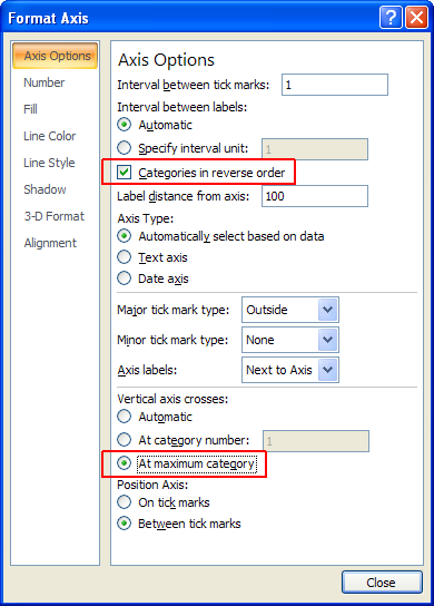
Excel Charts: Plotting Bar Chart Categories in Reverse Order
Order of Series and Legend Entries in Excel Charts - Peltier Tech Excel tries to place the same number of entries into each row: 8 entries in the original legend, then 4+4 entries, then 3+3+2, and finally 2+2+2+2. It's a little different with a vertically aligned legend. Below left is the same chart as above, with the legend listing the series along the right edge of the chart.

How to edit the label of a chart in Excel? - Stack Overflow
Edit titles or data labels in a chart - support.microsoft.com The first click selects the data labels for the whole data series, and the second click selects the individual data label. Right-click the data label, and then click Format Data Label or Format Data Labels. Click Label Options if it's not selected, and then select the Reset Label Text check box. Top of Page

How to Change Excel Chart Data Labels to Custom Values?
How to Customize Your Excel Pivot Chart Data Labels The Data Labels command on the Design tab's Add Chart Element menu in Excel allows you to label data markers with values from your pivot table. When you click the command button, Excel displays a menu with commands corresponding to locations for the data labels: None, Center, Left, Right, Above, and Below. None signifies that no data labels ...
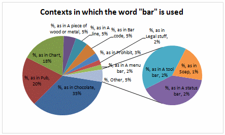
Automatically Group Smaller Slices in Pie Charts to one big Slice | Chandoo.org - Learn ...
Change the plotting order of categories, values, or data series Click the chart for which you want to change the plotting order of data series. This displays the Chart Tools. Under Chart Tools, on the Design tab, in the Data group, click Select Data. In the Select Data Source dialog box, in the Legend Entries (Series) box, click the data series that you want to change the order of.
Excel charts: add title, customize chart axis, legend and data labels
Legend label order and chart data series order do not correspond The Excel 2010 order of chart labels in our legend, does not match the order of the series in the 'Chart Data' dialog box. The entries in the chart legend are different than the series order in the 'Legend Entries (Series)' column of the 'Select Data Source' dialog. Changes to the order of the legend series in the 'Data Source' dialog are not ...
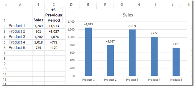
How-to Use Data Labels from a Range in an Excel Chart - Excel Dashboard Templates
Add or remove data labels in a chart - support.microsoft.com Click the data series or chart. To label one data point, after clicking the series, click that data point. In the upper right corner, next to the chart, click Add Chart Element > Data Labels. To change the location, click the arrow, and choose an option. If you want to show your data label inside a text bubble shape, click Data Callout.
How to make a bar graph in Excel
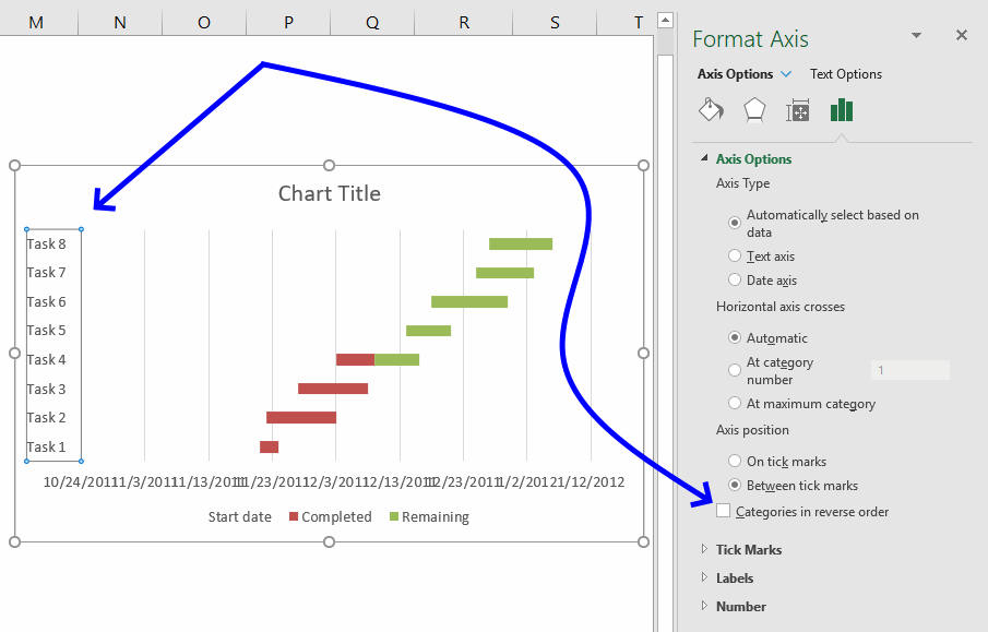
Excel tutorial: How to reverse a chart axis Luckily, Excel includes controls for quickly switching the order of axis values. To make this change, right-click and open up axis options in the Format Task pane. There, near the bottom, you'll see a checkbox called "values in reverse order". When I check the box, Excel reverses the plot order. Notice it also moves the horizontal axis to the ...

Enable or Disable Excel Data Labels at the click of a button - How To - PakAccountants.com
Change the Order of Data Series of a Chart in Excel - Excel Unlocked We can change this order. Right click on this chart and click on the Select Data option. After that select 2019 from the data series and click on the down arrow. This will move the data series 2019 below 2020. Click OK. As a result, you would see a change of order in your column chart as follows. This brings us to the end of the blog.
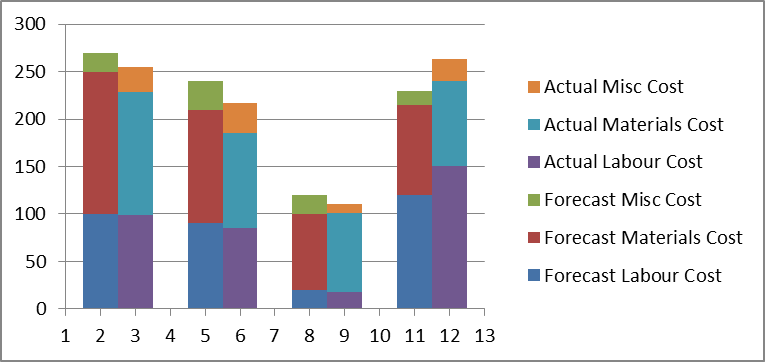
Step-by-step tutorial on creating clustered stacked column bar charts (for free) | Excel Help HQ
How to reorder chart series in Excel? - ExtendOffice Right click at the chart, and click Select Data in the context menu. See screenshot: 2. In the Select Data dialog, select one series in the Legend Entries (Series) list box, and click the Move up or Move down arrows to move the series to meet you need, then reorder them one by one. 3. Click OK to close dialog.
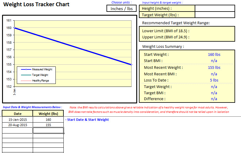
Weight Loss Chart Template
How to add or move data labels in Excel chart? - ExtendOffice In Excel 2013 or 2016. 1. Click the chart to show the Chart Elements button . 2. Then click the Chart Elements, and check Data Labels, then you can click the arrow to choose an option about the data labels in the sub menu. See screenshot: In Excel 2010 or 2007. 1. click on the chart to show the Layout tab in the Chart Tools group. See ...
How to Add Data Labels in an Excel Chart in Excel 2010 - YouTube

How to Make Excel Charts More Intuitive by Adding Data Labels and Tables - Data Recovery Blog
Excel Custom Chart Labels • My Online Training Hub
Advanced Gantt Chart Template
Post a Comment for "45 change order of data labels in excel chart"